French National Research Agency (ANR) in the framework of the HARWAVE project (ANR-23-CE47-0010)
Math
...
🚧 Site in progress
Help: Overlay microstrip
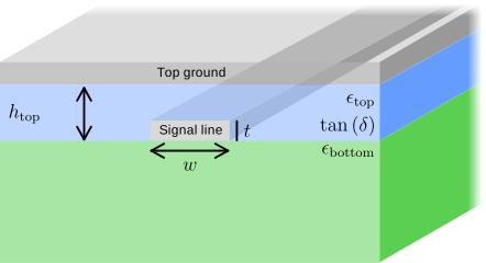
εtop, wafer dielectric permittivity
εbottom, top dielectric layer permittivity
htop, top dielectric layer thickness in µm
t, Metal thickness in nm
w, Metal width in µm
tan(δ), top dielectric layer loss tangent
Save project
Load project
Click to export your amplifier geometry into a netlist file adapted to
the Julia package "JosephsonCircuits.jl" by Kevin P. O'Brien and Maxime Malnou.
Click to load your simulation.
Click to save your simulation.
If checked, any change in the parameters will trigger a simulation. No need to click on the simulation button
anymore.
Relative dielectric permittivity of the substrate supporting the microstrip.
Higher values increase capacitance per unit of length.
Relative dielectric permittivity of the dielectric layer located between the signal line and the top ground
plane.
Higher values increase capacitance per unit of length.
Thickness of the substrate beneath the signal line.
Larger thickness generally reduces capacitance and increases characteristic impedance.
Thickness of the dielectric layer above the signal line.
Higher values decrease capacitance per unit of length.
Thickness of the superconducting signal line.
Width of the superconducting signal line.
Higher values increase capacitance per unit of length.
Dielectric loss tangent:
$\tan\left(\delta\right)=\mathrm{Im}\left(\epsilon\right)/\mathrm{Re}\left(\epsilon\right)$.
Higher values increase insertion losses.
Computed total amplifier length from all modulation sections.
Number of periodic modulation profiles combined for dispersion engineering.
Number of discretization points used to describe one period.
Higher values improve precision.
Number of repeated modulation periods.
Maximum positive width variation relative to nominal width.
Maximum negative width variation relative to nominal width.
Apply an envelope function to progressively reduce modulation amplitude
at both ends of the amplifier.
Controls transition length between tapered and flat regions.
Controls smoothness of the taper edges.
Desired sidelobe attenuation in dB.
Standard deviation of the Gaussian taper.
Controls taper shape and sidelobe suppression.
Controls taper shape and sidelobe suppression.
Fraction of the structure kept at full modulation.
Controls transition region size.
Fraction of the window occupied by cosine tapering.
Sheet kinetic inductance of the superconducting material.
Computed sheet kinetic inductance including current-induced nonlinearity.
If checked, the sheet kinetic inductance used in the computation of the Smatrix depends on the different current
as: $$L_\mathrm{k} = L_\mathrm{k0} \left( 1 + \left( \frac{I_\mathrm{p0} + I_\mathrm{dc}}{I^*} \right)^2
\right)$$.
Characteristic nonlinear current scale controlling inductance variation.
Internally, depairing current is used with: $I_\mathrm{d}=\frac{2}{3} I^*$
Pump current amplitude injected into the amplifier.
Pump frequency used for parametric amplification.
Optional DC bias current applied together with the RF pump.
Small signal current amplitude used to compute gain.
Add reflection to the boundary of the amplifier, see S. Kern et al. "Reflection-enhanced gain in traveling-wave parametric amplifiers" Phys. Rev. B 107, 174520 (2023)
Add white noise to the computed inductance and capacitance per unit of length. Both noise are added
independently.
Number of point along the amplifier used as step in the Coupled-Of-Mode equations.
Since the Runge-Kutta method is used, the actual number of step is not known.
This this parameter fixed the intial step as: $h_\mathrm{init} = \ell_\mathrm{amplifier}/\mathrm{Nb \; point}$
and the maximun number of step as: $\mathrm{Nb \; point}$.
Add loss factor by replaing the wavenumber $k$ by the complex propagation constant $\gamma = \alpha + \mathrm{i}\, k$.
Then each mode is
$$\partial_t I_\mathrm{a} = - \frac{k^2}{9 I_\mathrm{d}^2 \left( \alpha + \mathrm{i}\, k\right)} \left[ \cdots \right] + \frac{\alpha}{k - \mathrm{i} \, \alpha} \left(\mathrm{i}\frac{\alpha}{2} -k \right)I_\mathrm{a}$$.
Take into account the spatial dependence of some parameters :
Number of generated pump harmonics included in the solver.
1st: $3 \omega_\mathrm{p} = \omega_\mathrm{3p}$
Number of generated signal harmonics included in the solver.
1st: $3 \omega_\mathrm{s} = \omega_\mathrm{3s}$
Number of frequency sidebands included in coupled-mode equations.
1st: $\omega_\mathrm{s} + \omega_\mathrm{i1} = 2 \omega_\mathrm{p}$
2nd: $\omega_\mathrm{s} - \omega_\mathrm{i2} = -2 \omega_\mathrm{p}$
3rd: $\omega_\mathrm{s} + \omega_\mathrm{i3} = 4 \omega_\mathrm{p}$
Starting frequency of the simulation of the S matrix.
Ending frequency of the simulation of the S matrix.
Frequency resolution used for computation of the S matrix.
Starting frequency of the simulation of the Gain.
Ending frequency of the simulation of the Gain.
Frequency resolution used for computation of the Gain.
Choose which cost function is used to optimize the parameters.
Choose which parameters is being optimized.
Show the S11 and the S21 matrix components in dB a function of the signal frequency.
Show the k wavenumber, real and imag part, as a function of the signal frequency.
Show the modes gain in dB as function of the gain frequency.
You may shift the signal frequency vertical line to see at what frequencies the other bands are.
Show the width in μm of the amplifier along its length.
Show the characteristic impedance in Ω of the amplifier along its length.
Show the modes current in μA as function of the amplifier length.
Click to set a minimum value for the y-axis.
Desired characteristic impedance used during optimization.
Select which parameter is adjusted automatically to reach target impedance.